
When 88% Agreement Becomes 51%
Good diagnostic performance does not always produce a high kappa. A reproducible multi-reader simulation shows why prevalence matters — and why agreement analysis should go beyond a single coefficient.

A simple question with a surprising answer
Inter-reader agreement seems straightforward: if several clinicians evaluate the same cases, how often do they reach the same conclusion?
In practice, the answer depends heavily on how agreement is measured.
We created a reproducible multi-reader, multi-case simulation with:
500 cases,
5 readers,
2 reading sessions,
approximately 10% positive prevalence.
The simulated readers were deliberately set to perform well. Across repeated simulations, they achieved approximately 85% sensitivity and 95% specificity.
Observed inter-reader agreement was also high: around 88%.
Yet Fleiss’ kappa was only:
κ = 0.51
This is not a calculation error.
It is a property of how kappa defines agreement expected “by chance”.
High diagnostic performance does not necessarily imply a high kappa.
Why did kappa fall so low?
Kappa does not report the percentage of times readers agree.
Instead, it adjusts observed agreement for agreement that the method considers likely to occur by chance.
Conceptually:
Kappa = (Observed agreement − Expected chance agreement) / (1 − Expected chance agreement)
In our simulated dataset, observed agreement was approximately:
88.3%
But Fleiss’ method estimated expected chance agreement at approximately:
76.0%
Because negative ratings were much more common than positive ratings, two readers already had a high probability of giving the same classification purely from the marginal distribution of the categories.
After this adjustment, the final coefficient was only:
κ ≈ 0.51
This is a classic example of the so-called kappa prevalence paradox: high observed agreement can coexist with a surprisingly modest kappa when one outcome category dominates.
Importantly, a kappa of 0.51 does not mean that readers agreed in only 51% of cases.
They agreed in approximately 88%.
The 0.51 is a chance-corrected coefficient.

What happens with Gwet’s AC1?
We then applied Gwet’s AC1 to exactly the same reader ratings.
Nothing changed in the data.
Observed agreement remained:
88.3%
But Gwet’s AC1 was:
AC1 ≈ 0.85
The reason is simple: Gwet’s method defines expected chance agreement differently.
For the same dataset:
Fleiss’ expected chance agreement: 76.0%
Gwet’s expected chance agreement: 24.0%
The difference between κ = 0.51 and AC1 = 0.85 therefore does not come from different readers, different cases or different observed agreement.
It comes from the statistical definition of chance.
This does not mean that AC1 should automatically replace kappa in every analysis. But it does show why agreement coefficients should never be interpreted without understanding how they behave under the observed prevalence and category distribution.
The disagreement between kappa and AC1 is not about the data. It is about the definition of chance.
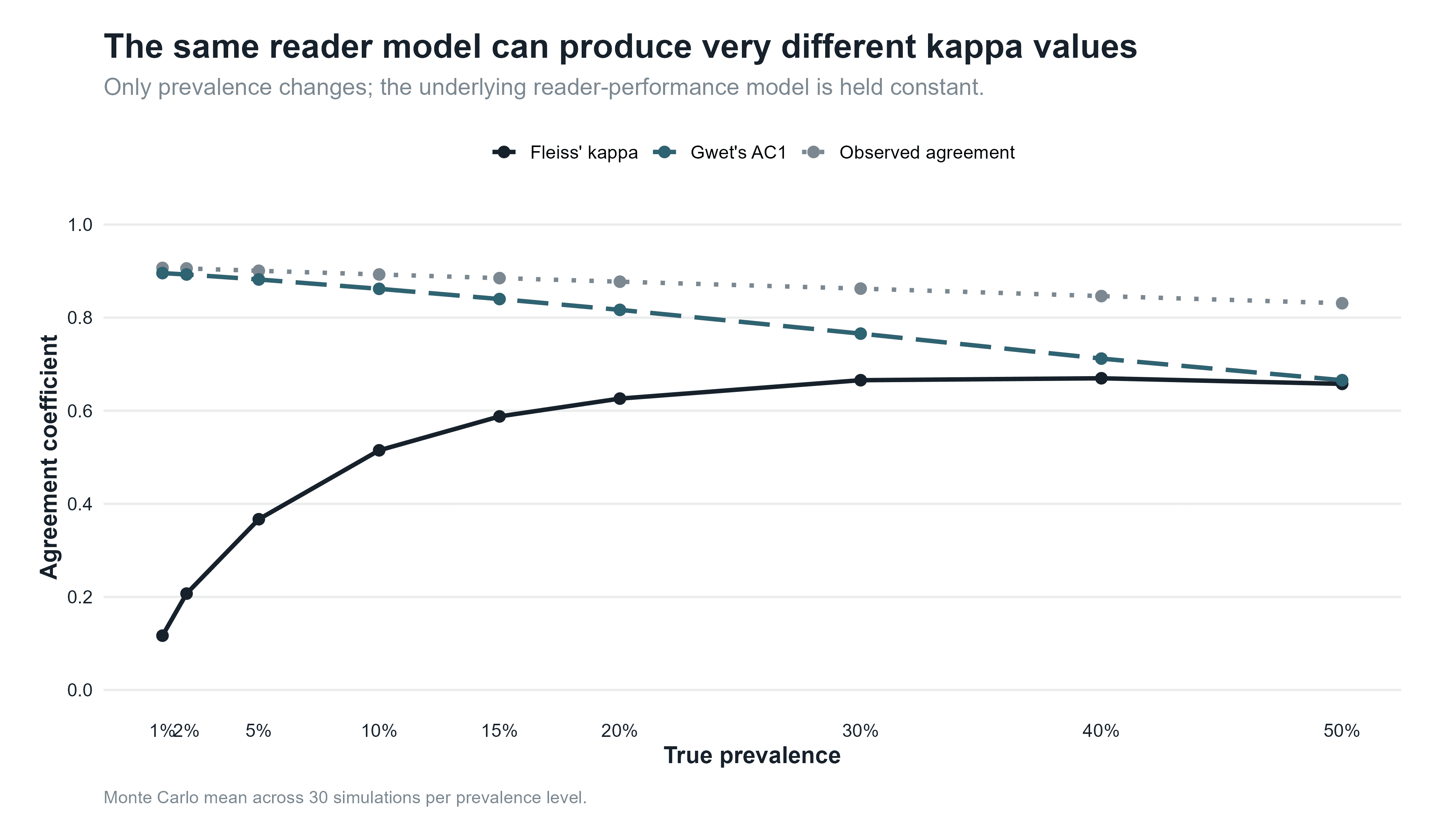
Prevalence can change the statistic without changing the reader
The advantage of simulation is that we know the underlying reader performance.
This allows us to perform a controlled experiment.
We can keep sensitivity, specificity and reader heterogeneity essentially unchanged while varying only the prevalence of positive cases.
That distinction is important.
Prevalence is a property of the population being evaluated.
It is not a property of the reader.
If changing prevalence substantially changes an agreement coefficient while the reader model remains unchanged, then the coefficient is reflecting more than reader reliability alone.
This is exactly what we investigate in the next step of the analysis.
By varying prevalence from balanced to highly unbalanced populations, we can compare how:
observed agreement,
Fleiss’ kappa,
Gwet’s AC1
respond to the same underlying reader model.
The result illustrates why two studies using readers with similar diagnostic performance can nevertheless report very different kappa values simply because their patient populations differ.

Inter-reader and intra-reader agreement are different
Our second reading session allows us to separate another pair of concepts.
Inter-reader agreement asks whether different readers classify the same case similarly.
Intra-reader agreement asks whether the same reader reproduces their own decision when the case is assessed again.
In our simulation, mean intra-reader agreement was approximately 93%, compared with approximately 89% inter-reader agreement.
This is a realistic pattern: readers can be more consistent with themselves than they are with each other.
It also shows why agreement analysis can benefit from moving beyond a single summary coefficient.
With richer models, disagreement can be decomposed into components associated with:
reader differences,
case difficulty,
repeated-reading variation,
reader-by-case interaction.
This turns agreement analysis from a descriptive exercise into an explanation of where uncertainty actually comes from.
The practical lesson
Our simulation produced a deliberately simple but important result:
Sensitivity ≈ 85%
Specificity ≈ 95%
Observed inter-reader agreement ≈ 88%
Fleiss’ κ ≈ 0.51
Gwet’s AC1 ≈ 0.85
All five statements are simultaneously true.
The apparent contradiction disappears once diagnostic accuracy, observed agreement and chance-corrected agreement are treated as different statistical concepts.
Kappa remains a useful statistic, but it should not be interpreted in isolation — especially when prevalence is low or category distributions are highly unbalanced.
For multi-reader studies, a better workflow is to examine observed agreement, prevalence and marginal distributions alongside the selected chance-corrected coefficient, and to consider alternatives such as Gwet’s AC1 where appropriate.